Before as_raw_html() was able to include images or custom styles like gtExtras::gt_theme_538() with inline CSS, it was a bit tricky to include tables in Quarto docs. I’ve spent some time trying to manually change all table classes in the html so that Quarto cannot overwrite it. Still, some stuff like line heights are still inherited from the surrounding Quarto doc (regardless of whether you use as_raw_html() or my function). I solved this issue by wrapping the code chunk into a div using style="all:initial;" (maybe there’s a more elegant solution).
In some cases, as_raw_html() does not seem to adjust line styles. Below, I’ve tested a few (non-minimal) table examples to see how the formatting may or may not change. In my examples, there were mainly two issues.
as_raw_html() still needs a surrounding div with style="all:initial;"
Small line heights lead to scroll bars that are not there when creating the table outside of Quarto
Line styles are not adjusted with as_raw_html().
1.1 My main function
The new as_raw_html() is probably preferable to my own function (as it likely won’t work with nested tables). But since my function does not have the issue with the line formatting I’ve kept it here for comparisons.
Code
make_tbl_quarto_robust <-function(tbl) {# Get tbl html code (without the inline stuff) tbl_html <- tbl |>as_raw_html(inline_css =FALSE) # Find table id tbl_id <-str_match(tbl_html, 'id="(.*)"\\s')[,2] # Split html so that we only replace strings in the css part at first# That's important for performance split_html <- tbl_html |>str_split_1('<table class="gt_table".{0,}>') css_part <- split_html[1] |>str_split_1('<style>')# Create regex to add table id my_regex <-str_c('(', tbl_id, ' )?(.* \\{)') replaced_css <- css_part[2] |># Make global html changes more specificstr_replace_all('html \\{', str_c(tbl_id, ' .gt_table {')) |># Make changes to everything specific to the table idstr_replace_all(my_regex, str_c('\\#', tbl_id, ' \\2')) |># Replace duplicate names str_replace_all(str_c('\\#', tbl_id, ' \\#', tbl_id),str_c('\\#', tbl_id) )# Put split html back togetherstr_c( css_part[1], '<style>', replaced_css, '<table class="gt_table">', split_html[2] ) |># Rename all gt_* classes to new_gt_*str_replace_all('(\\.|class="| )gt', '\\1new_gt') |># Reformat as htmlhtml()}
1.2 Line height issue
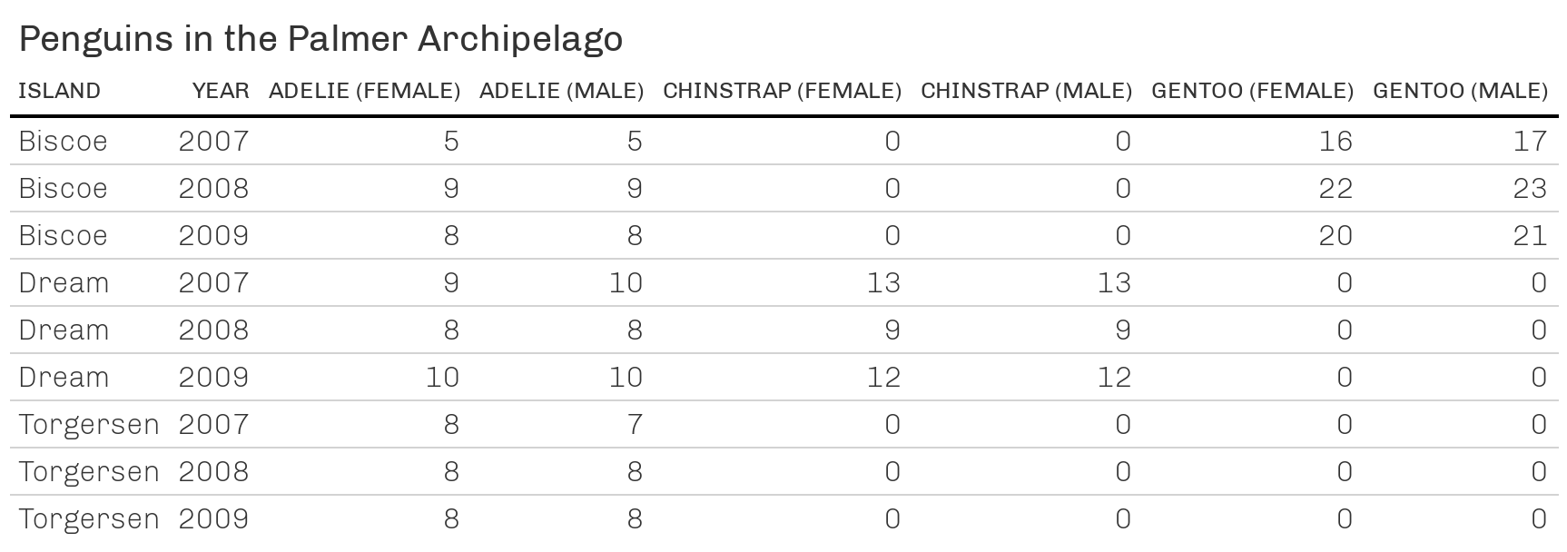
In this table, the line heights seem to still be inherited if we don’t wrap our div in style="all:initial;". Beware that the screenshoted table uses full width whereas the other tables are restricted to the page column of this Quarto doc.
Code
library(tidyverse)library(gt)library(gtExtras)penguins <- palmerpenguins::penguins |>filter(!is.na(sex))counts <- penguins |>mutate(year =as.character(year)) |>group_by(species, island, sex, year) |>summarise(n =n(), .groups ='drop')counts_wider <- counts |>pivot_wider(names_from =c(species, sex),values_from = n ) |>arrange(year) |># This will arrange each island as 07-08-09-totalmutate(island =paste('Island:', island)) |>ungroup()tbl <- counts_wider |>mutate(island =str_remove(island, 'Island: '),across(.cols =-(1:2), .fns =~replace_na(., replace =0)) ) |>arrange(island) |>gt(id ='asdsdag') |>cols_label('island'='Island',year ='Year',Adelie_female ='Adelie (female)',Adelie_male ='Adelie (male)',Chinstrap_female ='Chinstrap (female)',Chinstrap_male ='Chinstrap (male)',Gentoo_female ='Gentoo (female)',Gentoo_male ='Gentoo (male)', ) |>tab_header(title ='Penguins in the Palmer Archipelago') |>tab_options(heading.align ='left' ) |>gt_theme_538()
It seems that narrow line heights lead to scroll bars in all cases. The original table does not have that. Though, the initial table has full width and is not restricted. This may cause the issue?
Code
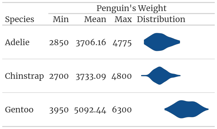
filtered_penguins <- palmerpenguins::penguins |>filter(!is.na(sex))penguin_weights <- palmerpenguins::penguins |>filter(!is.na(sex)) |>group_by(species) |>summarise(Min =min(body_mass_g),Mean =mean(body_mass_g) |>round(digits =2),Max =max(body_mass_g) ) |>mutate(species =as.character(species), Distribution = species) |>rename(Species = species)plot_density_species <-function(species, variable) { full_range <- filtered_penguins |>pull({{variable}}) |>range() filtered_penguins |>filter(species ==!!species) |>ggplot(aes(x = {{variable}}, y = species)) +geom_violin(fill ='dodgerblue4') +theme_minimal() +scale_y_discrete(breaks =NULL) +scale_x_continuous(breaks =NULL) +labs(x =element_blank(), y =element_blank()) +coord_cartesian(xlim = full_range)}penguins <- penguin_weights |>gt() |>tab_spanner(label ='Penguin\'s Weight',columns =-Species ) |>text_transform(locations =cells_body(columns ='Distribution'),# Create a function that takes the a column as input# and gives a list of ggplots as outputfn =function(column) {map(column, ~plot_density_species(., body_mass_g)) |>ggplot_image(height =px(50), aspect_ratio =3) } ) |>tab_options(table.font.names ='Merriweather') |>opt_css('.gt_table { line-height:10px; }' )
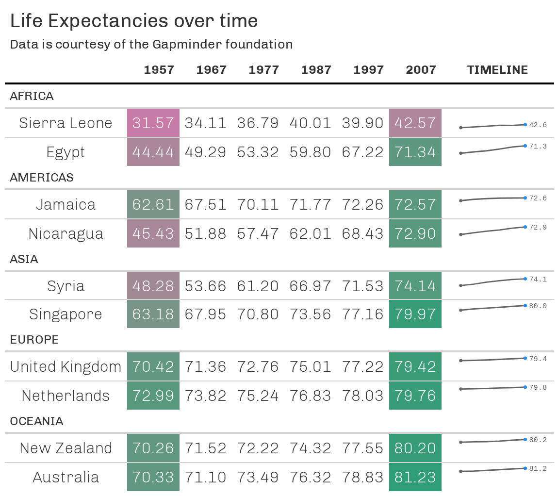
In all cases, the line between two countries looks thinner than in the screenshot. With as_raw_html() there is also a superfluous line below the last country in a continent.
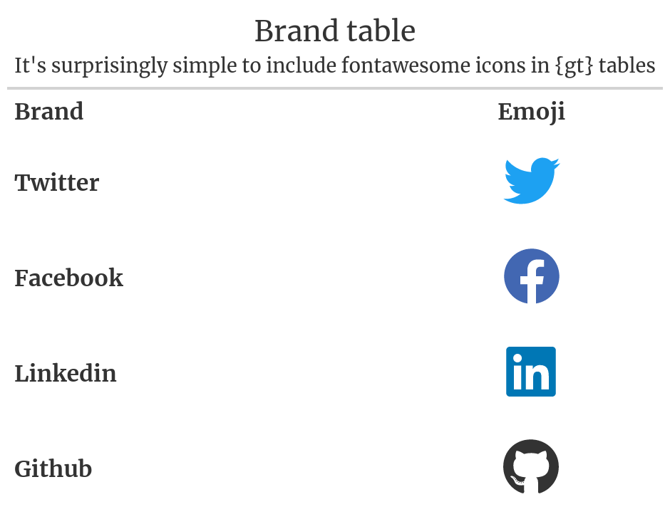
It's surprisingly simple to include fontawesome icons in {gt} tables
Brand
Emoji
Twitter
Facebook
Linkedin
Github
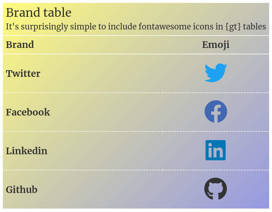
Brand table
It's surprisingly simple to include fontawesome icons in {gt} tables
Brand
Emoji
Twitter
Facebook
Linkedin
Github
Brand table
It's surprisingly simple to include fontawesome icons in {gt} tables
Brand
Emoji
Twitter
Facebook
Linkedin
Github
1.7 Body top-border can be fixed manually
Good news is that adding css code with opt_css() can fix most small issues I believe. Here that’s demonstrated with the previous body-top-border issue.